Site sections
Editor's Choice:
- Finland Largest Finnish city name
- The structure of secondary education in the United States
- Personal experience: my children study in Korea
- Scientists have reached a dead end, examining the mummy of Pirogov
- Thailand Population: Ethnic Composition, Occupations, Languages and Religion Thai Population Density
- Photo walk around the autumn academic city Where you can take a walk in the academic city
- How did it happen that four languages are spoken in Switzerland?
- Bosnian language Official language of Bosnia and Herzegovina
- Mozambique: a brief description of the country
- Almaty Document on renaming
Advertising
| Correlation coefficient. Pearson's correlation test Correlation coefficient 1 means |
|
» Statistics Statistics and data processing in psychology
|
|||||||||||||||||||||||||||||||||||||||||||||||||||||||||||||||||||||||||||||||||||||||||||||||||||||||||||||||||||||||||||||||||||||||||||||||||||||||||||||||||||||||||||||||||||||||||||||||||||||||||||||||||||||||||||||||||||||||||||||||||||||||||||||||||||||||||||||||||||||||||||||||||||||||||||||||||||||||||||||||||||||||||||||||||||||||||||||||||||||||||||||||||||||||||||||||||||||||||||||||||||||||||||||||||||||||||||||||||||||||||||||||||||||||||||||||||||||||||||||||||||||||


| Table 1. Criterion values t Student | |
| h | 0,05 |
| 1 | 6,31 |
| 2 | 2,92 |
| 3 | 2,35 |
| 4 | 2,13 |
| 5 | 2,02 |
| 6 | 1,94 |
| 7 | 1,90 |
| 8 | 1,86 |
| 9 | 1,83 |
| 10 | 1,81 |
| 11 | 1,80 |
| 12 | 1,78 |
| 13 | 1,77 |
| 14 | 1,76 |
| 15 | 1,75 |
| 16 | 1,75 |
| 17 | 1,74 |
| 18 | 1,73 |
| 19 | 1,73 |
| 20 | 1,73 |
| 21 | 1,72 |
| 22 | 1,72 |
| 23 | 1,71 |
| 24 | 1,71 |
| 25 | 1,71 |
| 26 | 1,71 |
| 27 | 1,70 |
| 28 | 1,70 |
| 29 | 1,70 |
| 30 | 1,70 |
| 40 | 1,68 |
| ¥ | 1,65 |
| Table 2. Values of the criterion χ 2 | |
| h | 0,05 |
| 1 | 3,84 |
| 2 | 5,99 |
| 3 | 7,81 |
| 4 | 9,49 |
| 5 | 11,1 |
| 6 | 12,6 |
| 7 | 14,1 |
| 8 | 15,5 |
| 9 | 16,9 |
| 10 | 18,3 |
| Table 3. Reliable Z values | |
| R | Z |
| 0,05 | 1,64 |
| 0,01 | 2,33 |
| Table 4. Reliable (critical) values of r | ||
| h =(N-2) | p= 0,05 (5%) | |
| 3 | 0,88 | |
| 4 | 0,81 | |
| 5 | 0,75 | |
| 6 | 0,71 | |
| 7 | 0,67 | |
| 8 | 0,63 | |
| 9 | 0,60 | |
| 10 | 0,58 | |
| 11 | 0.55 | |
| 12 | 0,53 | |
| 13 | 0,51 | |
| 14 | 0,50 | |
| 15 | 0,48 | |
| 16 | 0,47 | |
| 17 | 0,46 | |
| 18 | 0,44 | |
| 19 | 0,43 | |
| 20 | 0,42 | |
| Table 5. Reliable (critical) values of r s | |
| h =(N-2) | p = 0,05 |
| 2 | 1,000 |
| 3 | 0,900 |
| 4 | 0,829 |
| 5 | 0,714 |
| 6 | 0,643 |
| 7 | 0,600 |
| 8 | 0,564 |
| 10 | 0,506 |
| 12 | 0,456 |
| 14 | 0,425 |
| 16 | 0,399 |
| 18 | 0,377 |
| 20 | 0,359 |
| 22 | 0,343 |
| 24 | 0,329 |
| 26 | 0,317 |
| 28 | 0,306 |
7.3.1. Coefficients of correlation and determination. Can be quantified closeness of communication between factors and orientation(direct or reverse) by calculating:
1) if it is necessary to determine a linear relationship between two factors, - pair coefficient correlations: in 7.3.2 and 7.3.3, the operations of calculating the paired linear Bravais–Pearson correlation coefficient ( r) and Spearman's pairwise rank correlation coefficient ( r);
2) if we want to determine the relationship between two factors, but this relationship is clearly non-linear, then correlation relation ;
3) if we want to determine the relationship between one factor and some set of other factors - then (or, equivalently, "multiple correlation coefficient");
4) if we want to identify in isolation the relationship of one factor only with a specific other, which is part of a group of factors affecting the first, for which we have to consider the influence of all other factors unchanged, then private (partial) correlation coefficient .
Any correlation coefficient (r, r) cannot exceed 1 in absolute value, i.e. –1< r (r) < 1). Если получено значение 1, то это значит, что рассматриваемая зависимость не статистическая, а функциональная, если 0 - корреляции нет вообще.
The sign at the correlation coefficient determines the direction of the connection: the “+” sign (or the absence of a sign) means that the connection straight (positive), the “–” sign - that the connection reverse (negative). The sign has nothing to do with the tightness of the connection.
The correlation coefficient characterizes the statistical relationship. But often it is necessary to determine another type of dependence, namely: what is the contribution of a certain factor to the formation of another related factor. This kind of dependence, with a certain degree of conventionality, is characterized by determination coefficient (D ) determined by the formula D = r 2 ´100% (where r is the Bravais-Pearson correlation coefficient, see 7.3.2). If the measurements were taken in order scale (rank scale), then with some loss of reliability, instead of the value of r, the value of r (Spearman's correlation coefficient, see 7.3.3) can be substituted into the formula.
For example, if we obtained as a characteristic of the dependence of factor B on factor A the correlation coefficient r = 0.8 or r = –0.8, then D = 0.8 2 ´100% = 64%, that is, about 2 ½ 3. Therefore, the contribution of factor A and its changes to the formation of factor B is approximately 2 ½ 3 from the total contribution of all factors in general.
7.3.2. Bravais-Pearson correlation coefficient. The procedure for calculating the Bravais–Pearson correlation coefficient ( r ) can be used only in those cases when the connection is considered on the basis of samples having a normal frequency distribution ( normal distribution ) and obtained by measurements in scales of intervals or ratios. The calculation formula for this correlation coefficient is:
å ( x i – )( y i-)
r = .
n×sx×sy
What does the correlation coefficient show? Firstly, the sign at the correlation coefficient shows the direction of the relationship, namely: the “–” sign indicates that the relationship reverse, or negative(there is a trend: as the values of one factor decrease, the corresponding values of the other factor increase, and as they increase, they decrease), and the absence of a sign or the “+” sign indicates straight, or positive connections (there is a trend: with an increase in the values of one factor, the values of the other increase, and with a decrease, they decrease). Secondly, the absolute (sign-independent) value of the correlation coefficient indicates the tightness (strength) of the connection. It is customary to assume (rather conventionally): for values of r< 0,3 корреляция very weak, often it is simply not taken into account, for 0.3 £ r< 5 корреляция weak, for 0.5 £ r< 0,7) - average, at 0.7 £ r £ 0.9) - strong and, finally, for r > 0.9 - very strong. In our case (r » 0.83), the relationship is inverse (negative) and strong.
Recall that the values of the correlation coefficient can be in the range from -1 to +1. If the value of r goes beyond these limits, it indicates that in the calculations a mistake was made . If r= 1, this means that the connection is not statistical, but functional - which practically does not happen in sports, biology, medicine. Although with a small number of measurements, a random selection of values that gives a picture of a functional relationship is possible, but such a case is the less likely, the larger the volume of compared samples (n), that is, the number of pairs of compared measurements.
The calculation table (Table 7.1) is built according to the formula.
Table 7.1.
Calculation table for Bravais-Pearson calculation
| x i | y i | (x i-) | (x i – ) 2 | (y i-) | (y i – ) 2 | (x i – )( y i-) |
| 13,2 | 4,75 | 0,2 | 0,04 | –0,35 | 0,1225 | – 0,07 |
| 13,5 | 4,7 | 0,5 | 0,25 | – 0,40 | 0,1600 | – 0,20 |
| 12,7 | 5,10 | – 0,3 | 0,09 | 0,00 | 0,0000 | 0,00 |
| 12,5 | 5,40 | – 0,5 | 0,25 | 0,30 | 0,0900 | – 0,15 |
| 13,0 | 5,10 | 0,0 | 0,00 | 0,00 | 0.0000 | 0,00 |
| 13,2 | 5,00 | 0,1 | 0,01 | – 0,10 | 0,0100 | – 0,02 |
| 13,1 | 5,00 | 0,1 | 0,01 | – 0,10 | 0,0100 | – 0,01 |
| 13,4 | 4,65 | 0,4 | 0,16 | – 0,45 | 0,2025 | – 0,18 |
| 12,4 | 5,60 | – 0,6 | 0,36 | 0,50 | 0,2500 | – 0,30 |
| 12,3 | 5,50 | – 0,7 | 0,49 | 0,40 | 0,1600 | – 0,28 |
| 12,7 | 5,20 | –0,3 | 0,09 | 0,10 | 0,0100 | – 0,03 |
| åx i \u003d 137 \u003d 13.00 | åy i =56.1 =5.1 | å( x i - ) 2 \u003d \u003d 1.78 | å( y i – ) 2 = = 1.015 | å( x i – )( y i – )= = –1.24 |
Insofar as s x = ï ï = ï ï» 0.42, a
s y= ï ï» 0,32, r" –1,24ï (11´0.42´0.32) » –1,24ï 1,48 » –0,83 .
In other words, you need to know very firmly that the correlation coefficient can not exceed 1.0 in absolute value. This often makes it possible to avoid gross errors, or rather, to find and correct errors made in the calculations.
7.3.3. Spearman correlation coefficient. As already mentioned, it is possible to apply the Bravais-Pearson correlation coefficient (r) only in those cases when the analyzed factors are close to normal in terms of frequency distribution and the values of the variant are obtained by measurements necessarily on the scale of ratios or on the scale of intervals, which happens if they are expressed physical units. In other cases, the Spearman correlation coefficient is found ( r). However, this ratio can apply also in cases where it is allowed (and desirable ! ) apply the Bravais-Pearson correlation coefficient. But it should be borne in mind that the procedure for determining the Bravais-Pearson coefficient has more power ("resolving ability"), That's why r more informative than r. Even with a large n deviation r may be of the order of ±10%.
Table 7.2 Calculation formula for the coefficient
x i y i R x R y |d R | d R 2 Spearman correlation coefficient
13,2 4,75 8,5 3,0 5,5 30,25 r= 1 – . Vos
13.5 4.70 11.0 2.0 9.0 81.00 we use our example
12.7 5.10 4.5 6.5 2.0 4.00 for calculation r, but let's build
12.5 5.40 3.0 9.0 6.0 36.00 other table (Table 7.2).
13.0 5.10 6.0 6.5 0.5 0.25 Substitute the values:
13.2 5.00 8.5 4.5 4.0 16.00 r = 1– =
13,1 5,00 7,0 4,5 2,5 6,25 =1– 2538:1320 » 1–1,9 » – 0,9.
13.4 4.65 10.0 1.0 9.0 81.00 We see: r turned out to be a bit
12.4 5.60 2.0 11.0 9.0 81.00 more than r, but this is different
12.3 5.50 1.0 10.0 9.0 81.00 not very large. After all, at
12.7 5.20 4.5 8.0 3.5 12.25 so small n values r and r
åd R 2 = 423 are very approximate, not very reliable, their actual value can fluctuate widely, so the difference r and r in 0.1 is insignificant. Usuallyrconsidered as an analoguer , but less accurate. Signs at r and r shows the direction of the connection.
7.3.4. Application and validation of correlation coefficients. Determining the degree of correlation between factors is necessary to control the development of the factor we need: for this, we have to influence other factors that significantly affect it, and we need to know the measure of their effectiveness. It is necessary to know about the relationship of factors in order to develop or select ready-made tests: the information content of a test is determined by the correlation of its results with the manifestations of a trait or property of interest to us. Without knowledge of correlations, any form of selection is impossible.
It was noted above that in sports and in general pedagogical, medical, and even economic and sociological practice, it is of great interest to determine whether contribution , which the one factor contributes to the formation of another. This is due to the fact that in addition to the considered factor-causes on target(of interest to us) factor act, each giving one or another contribution to it, and others.
It is believed that the measure of the contribution of each factor-cause can be coefficient of determination D i = r 2 ´100%. So, for example, if r = 0.6, i.e. the relationship between factors A and B is average, then D = 0.6 2 ´100% = 36%. Knowing, therefore, that the contribution of factor A to the formation of factor B is approximately 1 ½ 3, it is possible, for example, to devote approximately 1 ½ 3 training times. If the correlation coefficient r \u003d 0.4, then D \u003d r 2 100% \u003d 16%, or approximately 1 ½ 6 - more than two times less, and according to this logic, only 1 should be given to its development ½ 6 part of training time.
The values of D i for various significant factors give an approximate idea of the quantitative relationship of their influences on the target factor of interest to us, for the sake of improving which we, in fact, are working on other factors (for example, a long jumper is working on increasing the speed of his sprint, so as it is the factor that makes the most significant contribution to the formation of the result in jumps).
Recall that by defining D instead of r put r, although, of course, the accuracy of the determination is lower.
Based selective(calculated from sample data) of the correlation coefficient, it is impossible to conclude that there is a connection between the considered factors in general. In order to draw such a conclusion with varying degrees of validity, use the standard correlation significance criteria. Their application assumes a linear relationship between the factors and normal distribution frequencies in each of them (meaning not a selective, but their general representation).
You can, for example, apply Student's t-tests. His race
even formula: tp= –2 , where k is the studied sample correlation coefficient, a n- the volume of compared samples. The resulting calculated value of the t-criterion (t p) is compared with the table value at the level of significance we have chosen and the number of degrees of freedom n = n - 2. To get rid of the calculation work, you can use a special table critical values of sample correlation coefficients(see above), corresponding to the presence of a significant relationship between the factors (taking into account n and a).
Table 7.3.
Boundary values of the reliability of the sample correlation coefficient
The number of degrees of freedom in determining the correlation coefficients is taken equal to 2 (i.e. n= 2) Indicated in the table. 7.3 values have a lower bound on the confidence interval true the correlation coefficient is 0, that is, with such values it cannot be argued that the correlation takes place at all. If the value of the sample correlation coefficient is higher than indicated in the table, it can be considered at the appropriate level of significance that the true correlation coefficient is not equal to zero.
But the answer to the question whether there is a real connection between the factors under consideration leaves room for another question: in what interval does true value correlation coefficient, as it can actually be, with an infinitely large n? This interval for any particular value r and n compared factors can be calculated, but it is more convenient to use a system of graphs ( nomogram), where each pair of curves constructed for some specified above them n, corresponds to the boundaries of the interval.
Rice. 7.4. Confidence limits of the sample correlation coefficient (a = 0.05). Each curve corresponds to the one above it. n.
Referring to the nomogram in Fig. 7.4, it is possible to determine the interval of values of the true correlation coefficient for the calculated values of the sample correlation coefficient at a = 0.05.
7.3.5. correlation relationships. If the pair correlation non-linear, it is impossible to calculate the correlation coefficient, determine correlation relationships . Mandatory requirement: features must be measured on a ratio scale or on an interval scale. You can calculate the correlation dependence of the factor X from the factor Y and correlation dependence of the factor Y from the factor X- they are different. With a small volume n considered samples representing factors, to calculate the correlation relationships, you can use the formulas:
correlation ratio h x ½ y= ;
correlation ratio h y ½ x= .
Here and are the arithmetic means of samples X and Y, and - intraclass arithmetic averages. That is, the arithmetic mean of those values in the sample of factor X, with which conjugate equal values in the sample of factor Y (for example, if factor X has values 4, 6, and 5, with which 3 options with the same value of 9 are associated in the sample of factor Y, then = (4+6+5) ½ 3 = 5). Accordingly, - the arithmetic mean of those values in the sample of the factor Y, which are associated with the same values in the sample of the factor X. Let's give an example and calculate:
X: 75 77 78 76 80 79 83 82 ; Y: 42 42 43 43 43 44 44 45 .
Table 7.4
Calculation table
| x i | y i | x y | x i – x | (x i – x) 2 | x i - x y | (x i–x y) 2 |
| –4 | –1 | |||||
| –2 | ||||||
| –3 | –2 | |||||
| –1 | ||||||
| –3 | ||||||
| x=79 | y=43 | S=76 | S=28 |
Therefore h y ½ x= » 0.63.
7.3.6. Partial and multiple correlation coefficients. To evaluate the relationship between 2 factors, by calculating the correlation coefficients, we assume by default that no other factors have any effect on this relationship. In reality, this is not the case. So, the relationship between weight and height is very significantly affected by the calorie intake, the amount of systematic physical activity, heredity, etc. When it is necessary when assessing the relationship between 2 factors take into account the significant impact other factors and at the same time how to isolate themselves from them, considering them unchanged, calculate private (otherwise - partial ) correlation coefficients.
Example: you need to evaluate paired dependencies between 3 essential factors X, Y and Z. Denote r XY (Z) private (partial) correlation coefficient between the factors X and Y (in this case, the value of the factor Z is considered unchanged), r ZX (Y) - partial correlation coefficient between the factors Z and X (with the constant value of the factor Y), r YZ (X) - partial correlation coefficient between the factors Y and Z (with the constant value of the factor X). Using the computed simple paired (according to Bravais-Pearson) correlation coefficients r xy, r XZ and r YZ, m
You can calculate private (partial) correlation coefficients using the formulas:
rXY- r XZ´ r YZ r XZ- r XY' r ZY r ZY –r ZX ´ r YZ
r XY (Z) = ; r XZ (Y) = ; r ZY (X) =
Ö(1– r 2XZ)(1– r 2 YZ) Ö(1– r 2XY)(1– r 2 ZY) Ö(1– r 2ZX)(1– r 2YX)
And partial correlation coefficients can take values from -1 to +1. By squaring them, we get the corresponding quotients determination coefficients also called private measures of certainty(multiplying by 100, we express in%%). Partial correlation coefficients differ more or less from simple (full) pair coefficients, which depends on the strength of the influence of the 3rd factor on them (as if unchanged). The null hypothesis (H 0), that is, the hypothesis that there is no connection (dependence) between factors X and Y, is tested (with the total number of features k) by calculating the t-test according to the formula: t P = r XY (Z) ´ ( n–k) 1 ½ 2 ´ (1– r 2XY(Z)) –1 ½ 2 .
If t R< t a n , the hypothesis is accepted (we assume that there is no dependence), if t P ³ t a n - the hypothesis is refuted, that is, it is believed that the dependence really takes place. t a n is taken from the table t-Student's criterion, and k- the number of factors taken into account (in our example 3), the number of degrees of freedom n= n - 3. Other partial correlation coefficients are checked similarly (into the formula instead of r XY (Z) are substituted accordingly r XZ (Y) or r ZY(X)).
Table 7.5
Initial data
| X (years) | Y (times) | Z (times) | X (years) | Y (times) | Z (times) | |||||||||||||||||
| Feature 1 Feature 2 | introversion | Extraversion |
| Sport games | a | b |
| Gymnastics | With | d |
Obviously, the numbers at our disposal here can only be distribution frequencies. In this case, calculate association coefficient (other name " contingency coefficient "). Consider the simplest case: the relationship between two pairs of features, while the calculated contingency coefficient is called tetrachoric (see table).
Table 7.7.
| a = 20 | b = 15 | a + b = 35 |
| c =15 | d=5 | c + d = 20 |
| a + c = 35 | b + d = 20 | n = 55 |
We make calculations according to the formula:
ad-bc 100-225-123
The calculation of association coefficients (conjugation coefficients) with a larger number of features is associated with calculations using a similar matrix of the corresponding order.
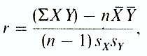
Pearson's correlation test is a parametric statistics method that allows you to determine the presence or absence of a linear relationship between two quantitative indicators, as well as evaluate its closeness and statistical significance. In other words, the Pearson correlation test allows you to determine whether there is a linear relationship between changes in the values of two variables. In statistical calculations and inferences, the correlation coefficient is usually denoted as rxy or Rxy.
1. History of the development of the correlation criterion
The Pearson correlation test was developed by a team of British scientists led by Karl Pearson(1857-1936) in the 90s of the 19th century, to simplify the analysis of the covariance of two random variables. In addition to Karl Pearson, Pearson's correlation test was also worked on Francis Edgeworth and Raphael Weldon.
2. What is Pearson's correlation test used for?
The Pearson correlation criterion allows you to determine what is the closeness (or strength) of the correlation between two indicators measured on a quantitative scale. With the help of additional calculations, you can also determine how statistically significant the identified relationship is.
For example, using the Pearson correlation criterion, one can answer the question of whether there is a relationship between body temperature and the content of leukocytes in the blood in acute respiratory infections, between the height and weight of the patient, between the content of fluoride in drinking water and the incidence of caries in the population.
3. Conditions and restrictions on the use of Pearson's chi-square test
- Comparable indicators should be measured in quantitative scale(for example, heart rate, body temperature, leukocyte count per 1 ml of blood, systolic blood pressure).
- By means of the Pearson correlation criterion, it is possible to determine only the presence and strength of a linear relationship between quantities. Other characteristics of the connection, including the direction (direct or reverse), the nature of the changes (rectilinear or curvilinear), as well as the dependence of one variable on another, are determined using regression analysis.
- The number of values to be compared must be equal to two. In the case of analyzing the relationship of three or more parameters, you should use the method factor analysis.
- Pearson's correlation criterion is parametric, in connection with which the condition for its application is normal distribution matched variables. If it is necessary to perform a correlation analysis of indicators whose distribution differs from the normal one, including those measured on an ordinal scale, Spearman's rank correlation coefficient should be used.
- It is necessary to clearly distinguish between the concepts of dependence and correlation. The dependence of the values determines the presence of a correlation between them, but not vice versa.
For example, the growth of a child depends on his age, that is, the older the child, the taller he is. If we take two children of different ages, then with a high degree of probability the growth of the older child will be greater than that of the younger. This phenomenon is called addiction, implying a causal relationship between indicators. Of course, there are also correlation, meaning that changes in one indicator are accompanied by changes in another indicator.
In another situation, consider the relationship between the growth of the child and the heart rate (HR). As you know, both of these values are directly dependent on age, therefore, in most cases, children of greater height (and therefore of older age) will have lower heart rate values. That is, correlation will be observed and may have a sufficiently high tightness. However, if we take children the same age, but different height, then, most likely, their heart rate will differ insignificantly, in connection with which we can conclude that independence Heart rate from growth.
The above example shows how important it is to distinguish between concepts fundamental in statistics connections and dependencies indicators to draw correct conclusions.
4. How to calculate the Pearson correlation coefficient?
Pearson's correlation coefficient is calculated using the following formula:

5. How to interpret the value of the Pearson correlation coefficient?
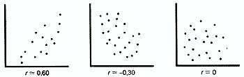
The values of the Pearson correlation coefficient are interpreted based on its absolute values. Possible values of the correlation coefficient vary from 0 to ±1. The greater the absolute value of r xy, the higher the closeness of the relationship between the two quantities. r xy = 0 indicates a complete lack of connection. r xy = 1 - indicates the presence of an absolute (functional) connection. If the value of the Pearson correlation criterion turned out to be greater than 1 or less than -1, an error was made in the calculations.
To assess the closeness, or strength, of the correlation, generally accepted criteria are used, according to which the absolute values of r xy< 0.3 свидетельствуют о weak connection, r xy values from 0.3 to 0.7 - about connection middle tightness, r xy values > 0.7 - o strong connections.
A more accurate estimate of the strength of the correlation can be obtained by using Chaddock table:
Grade statistical significance correlation coefficient r xy is carried out using the t-test, calculated by the following formula:
![]()
The obtained value t r is compared with the critical value at a certain level of significance and the number of degrees of freedom n-2. If t r exceeds t crit, then a conclusion is made about the statistical significance of the identified correlation.
6. An example of calculating the Pearson correlation coefficient
The aim of the study was to identify, determine the tightness and statistical significance of the correlation between two quantitative indicators: the level of testosterone in the blood (X) and the percentage of muscle mass in the body (Y). The initial data for a sample of 5 subjects (n = 5) are summarized in the table.
Correlation coefficients
Until now, we have found out only the very fact of the existence of a statistical relationship between two features. Next, we will try to find out what conclusions can be drawn about the strength or weakness of this dependence, as well as about its form and direction. Criteria for quantifying the relationship between variables are called correlation coefficients or measures of connectivity. Two variables are positively correlated if there is a direct, unidirectional relationship between them. In a unidirectional relationship, small values of one variable correspond to small values of the other variable, large values correspond to large ones. Two variables are negatively correlated if there is an inverse relationship between them. With a multidirectional relationship, small values of one variable correspond to large values of the other variable and vice versa. The values of the correlation coefficients are always in the range from -1 to +1.
As a correlation coefficient between variables belonging to ordinal scale applied Spearman's coefficient, and for variables belonging to interval scale - Pearson correlation coefficient(moment of works). It should be noted that each dichotomous variable, that is, a variable belonging to the nominal scale and having two categories, can be considered as ordinal.
First, we will check if there is a correlation between the sex and psyche variables from the studium.sav file. In this case, the dichotomous variable sex can be considered as ordinal. Do the following:
Select from the command menu Analyze (Analysis) Descriptive Statistics (Descriptive statistics) Crosstabs... (Tables of contingency)
Move variable sex to a list of strings, and a variable psyche- to the list of columns.
Click the button Statistics... (Statistics). In the Crosstabs: Statistics dialog, check the Correlations box. Confirm your choice with the Continue button.
In dialogue crosstabs Stop displaying tables by checking the Supress tables checkbox. Click the OK button.
The Spearman and Pearson correlation coefficients will be calculated, and their significance will be tested:
Symmetric Measures
| value | Asympt. Std. Error(a) (Asymptotic standard error) | Approx. T (b) (Approx. T) | Approx. Sig. (Approximate significance) | ||
| Interval by Interval (Interval - interval) | Pearson's R (R Pearson) |
,441 | ,081 | 5,006 | .000 (s) |
| Ordinal by Ordinal (Ordinal - Ordinal) | Spearman Correlation (Spearman Correlation) | ,439 | ,083 | 4,987 | .000 (s) |
| N of Valid Cases | 106 | ||||
Since there are no interval-scaled variables here, we will consider the Spearman correlation coefficient. It is 0.439 and is the most significant (p<0,001).
The following table is used to verbally describe the values of the correlation coefficient:
Based on the above table, the following conclusions can be drawn: There is a weak correlation between the variables sex and psyche (conclusion about the strength of dependence), the variables correlate positively (conclusion about the direction of dependence).
In the psyche variable, smaller values correspond to a negative mental state, and larger values correspond to a positive one. In the sex variable, in turn, the value "1" corresponds to the female gender, and "2" - male.
Consequently, the unidirectional relationship can be interpreted as follows: female students assess their mental state more negatively than male colleagues or, most likely, are more likely to agree to such an assessment when conducting a survey. When constructing such interpretations, one should take into account that the correlation between two traits is not necessarily the same as their functional or causal relationship, see Section 15.3 for more on this.
Now let's check the correlation between alter and semester variables. Let's apply the method described above. We will get the following coefficients:
Symmetric Measures
|
Asympt. Std. error(a) |
|||||
|
Interval by Interval |
|||||
|
Ordinal by Ordinal |
Spearman Correlation |
||||
|
N of Valid Cases |
|||||
a. Not assuming the null hypothesis (Null hypothesis is not accepted).
e. Using the asymptotic standard error assuming the null hypothesis.
With. Based on normal approximation.
Since alter and semester are metric variables, we will consider the Pearson coefficient (moment of products). It is 0.807. There is a strong correlation between alter and semester variables. The variables are positively correlated. Consequently, older students study in senior courses, which, in fact, is not an unexpected conclusion.
Let's check the variables sozial (assessment of social position) and psyche for correlation. We will get the following coefficients:
Symmetric Measures
|
Asympt. Std. error(a) |
|||||
|
Interval by Interval |
|||||
|
Ordinal by Ordinal |
Spearman Correlation |
||||
|
N of Valid Cases |
|||||
a. Not assuming the null hypothesis (Null hypothesis is not accepted).
b. Using the asymptotic standard error assuming the null hypothesis.
With. Based on normal approximation.
In this case, we will consider the Spearman correlation coefficient; it is -0.703. There is a moderate to strong correlation between sozial and psyche (cutoff 0.7). Variables are negatively correlated, that is, the greater the value of the first variable, the lower the value of the second and vice versa. Since small values of the variable sozial characterize a positive state (1 = very good, 2 = good), and large values of psyche characterize a negative state (1 = extremely unstable, 2 = unstable), therefore, psychological difficulties are largely due to social problems.
The correlation coefficient is the degree of association between two variables. Its calculation gives an idea of whether there is a relationship between two data sets. Unlike regression, correlation does not allow predicting values. However, the calculation of the coefficient is an important step in the preliminary statistical analysis. For example, we found that the correlation coefficient between the level of foreign direct investment and GDP growth is high. This gives us an idea that in order to ensure prosperity, it is necessary to create a favorable climate specifically for foreign entrepreneurs. Not so obvious conclusion at first glance!
Correlation and causation
Perhaps there is not a single area of statistics that would be so firmly established in our lives. The correlation coefficient is used in all areas of public knowledge. Its main danger lies in the fact that often its high values are speculated in order to convince people and make them believe in some conclusions. However, in fact, a strong correlation does not at all indicate a causal relationship between the quantities.

Correlation coefficient: Pearson and Spearman formula
There are several main indicators that characterize the relationship between two variables. Historically, the first is Pearson's linear correlation coefficient. It is passed at school. It was developed by K. Pearson and J. Yule based on the work of Fr. Galton. This coefficient allows you to see the relationship between rational numbers that change rationally. It is always greater than -1 and less than 1. A negative number indicates an inversely proportional relationship. If the coefficient is zero, then there is no relationship between the variables. Equal to a positive number - there is a directly proportional relationship between the studied quantities. Spearman's rank correlation coefficient makes it possible to simplify calculations by constructing a hierarchy of variable values.

Relationships between variables
Correlation helps answer two questions. First, whether the relationship between variables is positive or negative. Secondly, how strong is the addiction. Correlation analysis is a powerful tool with which to obtain this important information. It is easy to see that household incomes and expenses rise and fall proportionately. Such a relationship is considered positive. On the contrary, when the price of a product rises, the demand for it falls. Such a relationship is called negative. The values of the correlation coefficient are between -1 and 1. Zero means that there is no relationship between the studied values. The closer the indicator to the extreme values, the stronger the relationship (negative or positive). The absence of dependence is evidenced by a coefficient from -0.1 to 0.1. It must be understood that such a value only indicates the absence of a linear relationship.

Application features
The use of both indicators is subject to certain assumptions. First, the presence of a strong relationship does not determine the fact that one value determines the other. There may well be a third quantity that defines each of them. Secondly, a high Pearson correlation coefficient does not indicate a causal relationship between the studied variables. Thirdly, it shows an exclusively linear relationship. Correlation can be used to evaluate meaningful quantitative data (eg barometric pressure, air temperature) rather than categories such as gender or favorite color.
Multiple correlation coefficient
Pearson and Spearman investigated the relationship between two variables. But what to do if there are three or even more of them. This is where the multiple correlation coefficient comes in. For example, the gross national product is affected not only by foreign direct investment, but also by the monetary and fiscal policies of the state, as well as the level of exports. The growth rate and the volume of GDP are the result of the interaction of a number of factors. However, it should be understood that the multiple correlation model is based on a number of simplifications and assumptions. First, multicollinearity between quantities is excluded. Second, the relationship between the dependent variable and the variables that affect it is assumed to be linear.

Areas of use of correlation and regression analysis
This method of finding the relationship between quantities is widely used in statistics. It is most often resorted to in three main cases:
- For testing causal relationships between the values of two variables. As a result, the researcher hopes to find a linear relationship and derive a formula that describes these relationships between quantities. Their units of measurement may be different.
- To check for a relationship between values. In this case, no one determines which variable is dependent. It may turn out that the value of both quantities determines some other factor.
- To derive an equation. In this case, you can simply substitute numbers into it and find out the values of the unknown variable.
A man in search of a causal relationship
Consciousness is arranged in such a way that we definitely need to explain the events that occur around. A person is always looking for a connection between the picture of the world in which he lives and the information he receives. Often the brain creates order out of chaos. He can easily see a causal relationship where there is none. Scientists have to specifically learn to overcome this trend. The ability to evaluate relationships between data is objectively essential in an academic career.
Media bias
Consider how the presence of a correlation can be misinterpreted. A group of ill-behaved British students were asked if their parents smoked. Then the test was published in the newspaper. The result showed a strong correlation between parents' smoking and their children's delinquency. The professor who conducted this study even suggested putting a warning about this on cigarette packs. However, there are a number of problems with this conclusion. First, the correlation does not indicate which of the quantities is independent. Therefore, it is quite possible to assume that the pernicious habit of parents is caused by the disobedience of children. Secondly, it is impossible to say with certainty that both problems did not arise due to some third factor. For example, low-income families. It should be noted the emotional aspect of the initial conclusions of the professor who conducted the study. He was an ardent opponent of smoking. Therefore, it is not surprising that he interpreted the results of his study in this way.

conclusions
Misinterpreting correlation as a causal relationship between two variables can lead to embarrassing research errors. The problem is that it lies at the very core of human consciousness. Many marketing tricks are based on this feature. Understanding the difference between causation and correlation allows you to rationally analyze information both in everyday life and in your professional career.

New
- Spiritual wealth of a person
- Lesson on the world around on the topic "what is the world around"
- What does green mean What is green
- What is stress and how to deal with it?
- How to restore the nervous system and psyche at home Exercises for the human nervous system
- Pluto as a principle of transformation and rebirth of personality
- Restoration and strengthening of the nervous system and psyche at home What strengthens the nervous system
- Mental pain: three lessons for those who are now hard And what about self-medication
- Cainiao tracking in Russian Import clearance success Russian translation
- What will your fingerprints say?


