For the function of one variable y. = f.(x.) at point x. 0 the geometric meaning of the differential means the increment of the ordinate tangent, carried out to the graph of the function at the point with the abscissa x. 0 When switching to point x. 0 +  x.. And the differential function of two variables in this plan is increment applicatitangent planeconducted to the surface specified by the equation z. = f.(x., y.) , at point M. 0 (x. 0 , y. 0 ) when switching to point M.(x. 0 +  x., y. 0 +  y.). We give the definition of the tangent plane to some surface:

Df. . Plane passing through the point R 0 Surface S., called tangent planeat this point, if the angle between this plane and the sequential passing through two points R 0 and R(any surface point S.) tends to zero when the point Rseeks on this surface to the point R 0 .

Let the surface S.posted by equation z. = f.(x., y.). Then it can be shown that this surface has at the point P. 0 (x. 0 , y. 0 , z. 0 ) tangent plane then and only if the function z. = f.(x., y.) differential at this point. In this case, the tangent plane is given by the equation:

z. – z. 0 = +
(6).

§five. Derivative in direction, gradient function.

Partial derivatives functions y.= f.(x. 1 , x. 2 .. x. n. ) by variables x. 1 , x. 2 . . . x. n. Express the speed of changes in the direction of coordinate axes. For example, there is a speed change of function h. 1 - That is, it is assumed that the point belonging to the field definition area moves only parallel to the axis OH 1 And all other coordinates remain unchanged. However, it can be assumed that the function may vary in some other direction that does not coincide with the direction of any of the axes.

Consider the function of three variables: u.= f.(x., y., z.).

Fix point M. 0 (x. 0 , y. 0 , z. 0 ) and some directed straight (axis) l.passing through this point. Let be M (x., y., z.) - arbitrary point of this straight and  M. 0 M.- distance OT M. 0 before M.

u. = f. (x., y., z.) – f.(x. 0 , y. 0 , z. 0 ) - the increment of the function at the point M. 0 .

Find the ratio of the increment of the function to the length of the vector
:

Df. . Derived function u. = f. (x., y., z.) towards l. at point M. 0 Called the limit of the relationship of the increment function to the length of the vector M. 0 M. In the desire of the latter to 0 (or that the same, with an unlimited approximation M.to M. 0 ):

(1)

This derivative characterizes the speed of change of function at the point M. 0 in the direction l..

Let the axis l. (vector M. 0 M.) forms with axes OX., Oy., Oz.corners
respectively.

Denote x-x 0 \u003d
;

y - Y 0 \u003d
;

z - z 0 \u003d
.

Then vector M. 0 M \u003d (x. - x. 0 , y. - y. 0 , z. - z. 0 )=
and his guide cosines:

;

;

.

(4).

(4) - formula for calculating the derivative in the direction.

Consider the vector whose coordinates are private derived functions u.= f.(x., y., z.) at point M. 0 :

grad. u. - Gradient function u.= f.(x., y., z.) at point M (x., y., z.)

Gradient properties:

Output: Function gradient length u.= f.(x., y., z.) - there is the most affordable value at this point M (x., y., z.) , and the direction of the vector grad. u.coincides with the direction of the vector coming out of the point M., along which the function changes faster. That is, the direction of gradient function grad. u. - There is a direction of the definition of the function.

Tangent plane and normal surface.

tangent plane

Let N and N 0 be the points of this surface. We will spend direct nn 0. The plane that passes through the point N 0 is called tangent plane To the surface, if the angle between the unit nn 0 and this plane tends to zero when the distance nn 0 tends to zero.

Definition. Normalto the surface at point N 0 is the direct, passing through the point N 0 perpendicular to the tangent plane to this surface.

In some point, the surface has, or only one tangent plane or does not have it at all.

If the surface is set by the z \u003d f (x, y) equation, where f (x, y) is a function that is differentiable at the point m 0 (x 0, y 0), the tangent plane at point N 0 (x 0, y 0, ( x 0, y 0)) exists and has an equation:

The equation is normal to the surface at this point:

Geometric meaning The complete differential function of the two variables F (x, y) at the point (x 0, y 0) is the increment of applications (z coordinates) by the tangent plane to the surface when moving from point (x 0, y 0) to the point (x 0 +  , 0 + ).

As can be seen, the geometrical meaning of the complete differential function of two variables is the spatial analogue of the geometric meaning of the differential function of one variable.

Example. Find the equations of the tangent plane and normal to the surface

at point M (1, 1, 1).

The equation of the tangent plane:

Equation Normal:

20.4. Approximate calculations using a complete differential.

Let the function f (x, y) differ in the point (x, y). Find the full increment of this feature:

If we substitute expression into this formula

we will get an approximate formula:

Example. Calculate the approximate value, based on the value of the function, \u003d 1, y \u003d 2, z \u003d 1.

Of the specified expression, we define x \u003d 1.04 - 1 \u003d 0.04, y \u003d 1.99 - 2 \u003d -0.01,

z \u003d 1.02 - 1 \u003d 0.02.

Find the value of the function U (x, y, z) \u003d

Find private derivatives:

The full differential function U is equal:

The exact value of this expression: 1,049275225687319176.

20.5. Partial derivatives of higher orders.

If the function f (x, y) is defined in some region d, its private derivatives will be defined in the same area or part.

We will call these derivatives private first-order derivatives.

Derivatives of these functions will be second-order private derivatives.

Continuing to differentiate the equality obtained, we will receive private derivatives of higher orders.

Definition. Private derivatives species etc. called mixed derivatives.

Theorem. If the function f (x, y) and its private derivatives are determined and continuous at the point M (x, y) and its surroundings, then the ratio is true:

Those. Private derivatives of higher orders do not depend on the procedure for differentiation.

Similarly, the differentials of higher orders are determined.

…………………

Here n is a symbolic degree of the derivative, which is replaced by a real degree after the construction of the expression standing in it.

Differential calculus of functions of several variables.

Basic concepts and definitions.

When considering the functions of several variables, we will limit the detailed description of the functions of two variables, because All results obtained will be valid for the functions of an arbitrary number of variables.

If each pair of independent numbers (x, y) from a certain set of any rule is placed in accordance with one or more values \u200b\u200bof the variable z, then the variable Z is called the function of two variables.

If the pair of numbers (x, y) corresponds to one value z, then the function is called unambiguous, and if more than one, then - multivalued.

Definition area Functions Z is called a set of pairs (x, y), in which the function z exists.

Neighborhood pointM 0 (x 0, y 0) Radius R is called the totality of all points (x, y), which satisfy the condition.

The number is called limit Functions f (x, y) when the point of the point M (x, y) to the point m 0 (x 0, y 0), if for each number E\u003e 0 there is such a number R\u003e 0, which is for any point M (x, y), for which the condition is true

also true and condition .

Record:

Let the point M 0 (x 0, y 0) belongs to the field of determining the function f (x, y). Then the function z \u003d f (x, y) is called continuous At point m 0 (x 0, y 0), if

(1)

moreover, the point M (x, y) tends to point M 0 (x 0, y 0) an arbitrary manner.

If at some point condition (1) is not executed, then this point is called spray pointfunctions f (x, y). This may be in the following cases:

1) The function z \u003d f (x, y) is not defined at the point M 0 (x 0, y 0).

2) There is no limit.

3) This limit exists, but it is not equal to f (x 0, y 0).

Properties of functions of several variables associated with their continuity.

Property. If the function f (x, y, ...) is defined and continuous in a closed and limited area d, there is at least one point in this area.

N (x 0, y 0, ...), such that for other points is true inequality

f (x 0, y 0, ...) ³ f (x, y, ...)

as well as point n 1 (x 01, y 01, ...), such that for all other points is faithful inequality

f (x 01, y 01, ...) £ f (x, y, ...)

then f (x 0, y 0, ...) \u003d m - the greatest value functions, and f (x 01, y 01, ...) \u003d m - the smallest valuefunctions f (x, y, ...) in the region D.

The continuous function in a closed and limited area D reaches at least once the greatest value and once the smallest.

Property. If the function f (x, y, ...) is defined and continuous in a closed limited region D, and M and M - respectively, the largest and smallest values \u200b\u200bof the function in this area, then there is a point for any point M î

N 0 (x 0, y 0, ...) such that f (x 0, y 0, ...) \u003d m.

Simply put, the continuous function takes all intermediate values \u200b\u200bbetween M and m in the region D. The consequence of this property can be the conclusion that if the numbers M and M of different characters, then in the D region, the function at least once appeals to zero.

Property. Function f (x, y, ...), continuous in a closed limited area D, limited In this area, if there is such a number to that for all points of the region, inequality is true .

Property. If the function f (x, y, ...) is defined and continuous in a closed limited area D, then it uniformly continuous In this area, i.e. For any positive number E, there is such a number D\u003e 0, which for any two points (x 1, y 1) and (x 2, in 2) areas located at a distance of less d, inequality

2. Private derivatives. Partial derivatives of higher orders.

Suppose in some region, the function z \u003d f (x, y) is set. Take an arbitrary point M (x, y) and set the increment of DX to the variable x. Then the value of D x z \u003d f (x + dx, y) - f (x, y) is called private increment of function by x.

Can be recorded

.

Then called private derivativethe functions z \u003d f (x, y) by x.

Designation:

Similarly, a private derivative of functions of software is determined.

Geometric meaninga private derivative (for example) is the tangent of the tilt angle of tangent, carried out at point N 0 (x 0, y 0, z 0) to the surface cross section of the plane y \u003d y 0.

If the function f (x, y) is defined in some region d, its private derivatives will also be defined in the same area or part of it.

We will call these derivatives private first-order derivatives.

Derivatives of these functions will be second-order private derivatives.

Continuing to differentiate the equality obtained, we will receive private derivatives of higher orders.

Private derivatives species etc. called mixed derivatives.

Theorem. If the function f (x, y) and its private derivatives are determined and continuous at the point M (x, y) and its surroundings, then the ratio is true:

Those. Private derivatives of higher orders do not depend on the procedure for differentiation.

Similarly, the differentials of higher orders are determined.

…………………

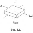
Here n is a symbolic degree of the derivative, which is replaced by a real degree after the construction of the expression standing in it.

FULL DIFFERENTIAL. The geometric meaning of the complete differential. Tangent plane and normal surface.

The expression is called full incrementfunctions f (x, y) at some point (x, y), where a 1 and a 2 are infinitely small functions with DX ® 0 and DU ® 0, respectively.

Complete differentialthe functions z \u003d f (x, y) are called the main linear part relative to the DX and DU of the increment of the function dz at the point (x, y).

For the function of an arbitrary number of variables:

Example 3.1.. Find a full differential function.

The geometrical meaning of the complete differential function of the two variables f (x, y) at the point (x 0, y 0) is the increment of applications (z coordinates) by the tangent plane to the surface when moving from point (x 0, y 0) to the point (x 0 + DX, in 0 + DU).

Partial derivatives of higher orders. :If the function f (x, y) is defined in some region d, its private derivatives will also be defined in the same area or part of it. We will call these derivatives of first-order private derivatives.

Derivatives of these functions will be partial derivatives of the second order.

Continuing to differentiate the equality obtained, we will receive private derivatives of higher orders. Definition. Private derivatives species etc. Called mixed derivatives. Schwartz theorem:

If private derivatives of higher orders F.M.P. Continuous, then mixed derivatives of one order, differing only by the procedure for differentiation \u003d each other.

Here n is a symbolic degree of the derivative, which is replaced by a real degree after the construction of the expression standing in it.

14. The equation of the tangent plane and normal to the surface!

Let N and N 0 be the points of this surface. We will spend direct nn 0. The plane that passes through the point N 0 is called tangent plane To the surface, if the angle between the unit nn 0 and this plane tends to zero when the distance nn 0 tends to zero.

Definition. Normalto the surface at point N 0 is the direct, passing through the point N 0 perpendicular to the tangent plane to this surface.

In some point, the surface has, or only one tangent plane or does not have it at all.

If the surface is set by the equation z \u003d f (x, y), where f (x, y) is a function that is differentiable at the point m 0 (x 0, y 0), tangent plane At point N 0 (x 0, y 0, (x 0, y 0)) exists and has an equation:

The equation is normal to the surface at this point.:

Geometric meaning The full differential function of the two variables f (x, y) at the point (x 0, y 0) is the increment of applications (coordinates z) of the tangent plane to the surface when moving from point (x 0, y 0) to the point (x 0 + dx, In 0 + DU).

As can be seen, the geometrical meaning of the complete differential function of two variables is the spatial analogue of the geometric meaning of the differential function of one variable.

16. The scalar field and its characteristics. Line ulni, derivatives in the direction, gradient of the scalar field.

If each point of space is put in accordance with the scalar value, the scalar field occurs (for example, temperature field, electric potential field). If the Cartesian coordinates are introduced, it is also denoted or The field can be flat, if the central (spherical) if cylindrical, if

Surfaces and Line: The properties of scalar fields can be visually studied using level surfaces. This surfaces in the space on which it takes a constant value. Their equation: . In a flat scalar field, the level lines call the curves on which the field takes constant value: In some cases, the level line can degenerate into the point, and the surface surfaces in the point and curves.

The derivative in the direction and gradient of the scalar field:

Let a single vector with coordinates - a scalar field. The derivative in the direction characterizes the change in the field in this direction and is calculated by the derivative formula in the direction is the scalar product of the vector and the vector with coordinates which is called a gradient function and is indicated. Communication where the angle between and, then the vector indicates the direction of the speedy increase in the field and its module is equal to the derivative in this direction. Since the gradient components are partial derivatives, it is not difficult to obtain the following gradient properties:

17. Extremes F.M.P. Blind Extremum F.M., necessary and sufficient conditions for its existence. The greatest and smallest value of F.M.P. In Ogran. closed area.

Let the function z \u003d ƒ (x; y) are defined in some region D, point n (x0; y0)

Point (x0; u0) is called the maximum point of the function z \u003d ƒ (x; y), if there is such a d-neighborhood of the point (x0; u0), which is for each point (x; y), other than (ho; uh), From this neighborhood, inequality ƒ (x; y)<ƒ(хо;уо). Аналогично определяется точка минимума функции: для всех точек (х; у), отличных от (х0;у0), из d-окрестности точки (хо;уо) выполняется неравенство: ƒ(х;у)>ƒ (x0; u0). The value of the function at the maximum point (minimum) is called a maximum (minimum) function. Maximum and minimum features are called its extremes. Note that, by the definition, the extremum point of the function lies inside the function of determining the function; Maximum and minimum have a local (local) character: the value of the function at the point (x0; U0) is compared with its values \u200b\u200bat points close to (x0; u0). In the D region, the function may have several extremums or have no one.

Required (1) and sufficient (2) conditions of existence:

(1) If at point n (x0; y0), the differential function z \u003d ƒ (x; y) has an extremum, then its private derivatives at this point are zero: ƒ "x (x0; y0) \u003d 0, ƒ" y (x0; y0 ) \u003d 0. Comment. The function may have an extremum at points where at least one of the partial derivatives does not exist. The point in which the private derivatives of the first order of the function z ≈ ƒ (x; y) are zero, i.e. f "x \u003d 0, f" y \u003d 0, is called the stationary point of the function z.

Stationary points and points in which at least one private derivative does not exist are called critical points

(2) Suppose in a stationary point (ho; uh) and some of its surroundings, the function ƒ (x; y) has continuous private derivatives to second order inclusive. Calculate at the point (x0; u0) the values \u200b\u200ba \u003d f "" xx (x0; y0), B \u003d ƒ "" xy (x0; u0), c \u003d ƒ "" oy (x0; u0). Denote Then:

1. If δ\u003e 0, then the function ƒ (x; y) at the point (x0; u0) has an extremum: maximum, if a< 0; минимум, если А > 0;

2. If Δ.< 0, то функция ƒ(х;у) в точке (х0;у0) экстремума не имеет.

3. In the case δ \u003d 0 extremum at the point (x0; u0) may not be. Additional research is needed.

$ E \\ Subset \\ Mathbb (R) ^ (n) $. It is said that $ F $ has local maximum At point $ x_ (0) \\ in E $, if there is such a neighborhood of $ U $ points $ x_ (0) $, that for all $ X \\ in U $, an inequality is $ f \\ left (x \\ right) \\ leqslant f \\ left (x_ (0) \\ Right) $.

Local maximum called strict If the neighborhood of $ u $ can be chosen so that for all $ x \\ in u $, different from $ x_ (0) $, there was $ F \\ Left (X \\ Right)< f\left(x_{0}\right)$.

Definition
Let $ F $ be the actual function on an open set $ E \\ Subset \\ Mathbb (R) ^ (n) $. It is said that $ F $ has local minimum At point $ x_ (0) \\ in E $, if there is such a neighborhood of $ U $ points $ x_ (0) $, that for all $ x \\ in U $, an inequality of $ F \\ Left (X \\ Right) \\ GEQSLANT F \\ left (x_ (0) \\ Right) $.

The local minimum is called strict if the neighborhood of $ U $ can be chosen so that for all $ x \\ in u $, different from $ x_ (0) $, there was $ F \\ Left (X \\ Right)\u003e F \\ Left (X_ ( 0) \\ Right) $.

Local extremum combines the concepts of a local minimum and a local maximum.

Theorem (the required condition of the extremum differentiable function)
Let $ F $ be the actual function on an open set $ E \\ Subset \\ Mathbb (R) ^ (n) $. If at point $ x_ (0) \\ in E $, the $ F function has a local extremum and at this point, then $$ \\ Text (D) F \\ Left (x_ (0) \\ Right) \u003d 0. $$ Equality zero The differential is equivalent to the fact that all are zero, i.e. $$ \\ DISPLAYSTYLE \\ FRAC (\\ Partial F) (\\ Partial x_ (i)) \\ left (x_ (0) \\ right) \u003d 0. $$

In the one-dimensional case it is. Denote by $ \\ phi \\ left (t \\ right) \u003d f \\ left (x_ (0) + th \\ right) $, where $ h $ is an arbitrary vector. The function $ \\ phi $ is defined with sufficiently small modulo values \u200b\u200bof $ t $. In addition, according to, it is differentiable, and $ (\\ phi) '\\ left (T \\ Right) \u003d \\ Text (D) F \\ Left (x_ (0) + Th \\ Right) H $.
Let $ F $ have a local maximum at $ 0 $ point. It means that the function $ \\ Phi $ with $ T \u003d 0 $ has a local maximum and, according to the farm theorem, $ (\\ phi) '\\ left (0 \\ right) \u003d 0 $.
So, we got that $ df \\ left (x_ (0) \\ right) \u003d 0 $, i.e. Functions $ F $ At point $ x_ (0) $ is zero on any vector $ H $.

Definition
Points in which the differential is zero, i.e. Such in which all private derivatives are zero, are called stationary. Critical points The functions of $ F $ are called such points in which $ F $ is not differentiated or equal to zero. If the point is stationary, then it does not yet follow that at this point the function has an extremum.

Example 1.
Let $ f \\ left (x, y \\ right) \u003d x ^ (3) + y ^ (3) $. Then $ \\ displaystyle \\ FRAC (\\ Partial F) (\\ Partial x) \u003d 3 \\ CDOT X ^ (2) $, $ \\ displaystyle \\ FRAC (\\ Partial F) (\\ Partial y) \u003d 3 \\ Cdot y ^ (2 ) $, so $ \\ left (0.0 \\ Right) $ is a stationary point, but at this point the function does not have an extremum. Indeed, $ F \\ Left (0.0 \\ Right) \u003d 0 $, but it is easy to see that in any neighborhood of the $ \\ left point (0.0 \\ RIGHT) $ function takes both positive and negative values.

Example 2.
The function is $ F \\ left (x, y \\ right) \u003d x ^ (2) - y ^ (2) $ start - stationary point, but it is clear that there is no extremum at this point.

Theorem (sufficient extremum condition).
Let the function $ F $ double-continuously differentiable on an open set $ E \\ Subset \\ MathBB (R) ^ (N) $. Let $ x_ (0) \\ in E $ - a stationary point and $$ \\ displaystyle q_ (x_ (0)) \\ left (h \\ right) \\ Equiv \\ Sum_ (i \u003d 1) ^ n \\ Sum_ (J \u003d 1) ^ n \\ FRAC (\\ Partial ^ (2) f) (\\ Partial x_ (i) \\ Partial x_ (j)) \\ left (x_ (0) \\ right) h ^ (i) H ^ (J). $$ Then

1. if $ q_ (x_ (0)) $ -, then the function $ F $ at $ x_ (0) $ has a local extremum, namely, at a minimum, if the form is positively defined, and the maximum, if the form is negatively defined;
2. if the quadratic form $ q_ (x_ (0)) $ is indefinite, then the function $ F $ at $ x_ (0) $ does not have an extremum.

We use the decomposition by the Taylor formula (12.7 p. 292). Considering that the individual derivatives of the first order at point $ x_ (0) $ are zero, we get $$ \\ displaystyle f \\ left (x_ (0) + h \\ right) -f \\ left (x_ (0) \\ right) \u003d \\ \\ left (x_ (0) + \\ theta h \\ right) h ^ (i) H ^ (J), $$ where $ 0<\theta<1$. Обозначим $\displaystyle a_{ij}=\frac{\partial^{2} f}{\partial x_{i} \partial x_{j}} \left(x_{0}\right)$. В силу теоремы Шварца (12.6 стр. 289-290) , $a_{ij}=a_{ji}$. Обозначим $$\displaystyle \alpha_{ij} \left(h\right)=\frac{\partial^{2} f}{\partial x_{i} \partial x_{j}} \left(x_{0}+\theta h\right)−\frac{\partial^{2} f}{\partial x_{i} \partial x_{j}} \left(x_{0}\right).$$ По предположению, все непрерывны и поэтому $$\lim_{h \rightarrow 0} \alpha_{ij} \left(h\right)=0. \left(1\right)$$ Получаем $$\displaystyle f \left(x_{0}+h\right)−f \left(x_{0}\right)=\frac{1}{2}\left.$$ Обозначим $$\displaystyle \epsilon \left(h\right)=\frac{1}{|h|^{2}}\sum_{i=1}^n \sum_{j=1}^n \alpha_{ij} \left(h\right)h_{i}h_{j}.$$ Тогда $$|\epsilon \left(h\right)| \leq \sum_{i=1}^n \sum_{j=1}^n |\alpha_{ij} \left(h\right)|$$ и, в силу соотношения $\left(1\right)$, имеем $\epsilon \left(h\right) \rightarrow 0$ при $h \rightarrow 0$. Окончательно получаем $$\displaystyle f \left(x_{0}+h\right)−f \left(x_{0}\right)=\frac{1}{2}\left. \left(2\right)$$ Предположим, что $Q_{x_{0}}$ – положительноопределенная форма. Согласно лемме о положительноопределённой квадратичной форме (12.8.1 стр. 295, Лемма 1) , существует такое положительное число $\lambda$, что $Q_{x_{0}} \left(h\right) \geqslant \lambda|h|^{2}$ при любом $h$. Поэтому $$\displaystyle f \left(x_{0}+h\right)−f \left(x_{0}\right) \geq \frac{1}{2}|h|^{2} \left(λ+\epsilon \left(h\right)\right).$$ Так как $\lambda>0 $, and $ \\ epsilon \\ left (H \\ Right) \\ RightarRow 0 $ with $ H \\ Rightarrow 0 $, then the right side will be positive with any vector $ H $ sufficiently small length.
So, we came to the fact that in some neighborhood of the point $ x_ (0) $ it was the inequality of $ f \\ left (x \\ right)\u003e F \\ left (x_ (0) \\ right) $, if only $ x \\ neq x_ (0) $ (we put $ x \u003d x_ (0) + h $ \\ right). This means that at point $ x_ (0) $ function has a strict local minimum, and thus proved the first part of our theorem.
Suppose now that $ q_ (x_ (0)) $ is an indefinite form. Then there are vectors $ H_ (1) $, $ H_ (2) $, such as $ Q_ (x_ (0)) \\ left (H_ (1) \\ Right) \u003d \\ lambda_ (1)\u003e 0 $, $ Q_ (x_ (0)) \\ left (H_ (2) \\ RIGHT) \u003d \\ Lambda_ (2)<0$. В соотношении $\left(2\right)$ $h=th_{1}$ $t>0 $. Then we get $$ f \\ left (x_ (0) + th_ (1) \\ right) -f \\ left (x_ (0) \\ right) \u003d \\ FRAC (1) (2) \\ left [t ^ (2) \\ left [\\ lambda_ (1) + | h_ (1) | ^ (2) \\ Epsilon \\ left (TH_ (1) \\ RIGHT) \\ Right]. $$ with sufficiently small $ T\u003e 0 $ The right-hand part is positive. This means that in any neighborhood of the point $ x_ (0) $, the $ F $ function takes the values \u200b\u200bof $ F \\ left (x \\ right) $, large than $ F \\ left (x_ (0) \\ Right) $.
Similarly, we obtain that in any neighborhood of the point $ x_ (0) $ function $ F $ takes the values \u200b\u200bless than $ F \\ left (x_ (0) \\ right) $. This, along with the previous one, means that at point $ x_ (0) $ function $ F $ does not have an extremum.

Consider a particular case of this theorem for the function $ F \\ left (x, y \\ right) $ two variables defined in some neighborhood of the $ \\ left point (x_ (0), y_ (0) \\ right) $ and in this neighborhood of continuous Private derivatives of the first and second orders. Suppose that $ \\ left (x_ (0), y_ (0) \\ right) $ is a stationary point, and denote $$ \\ displayStyle A_ (11) \u003d \\ FRAC (\\ Partial ^ (2) f) (\\ Partial x ^ (2)) \\ left (x_ (0), y_ (0) \\ Right), A_ (12) \u003d \\ FRAC (\\ Partial ^ (2) f) (\\ Partial x \\ Partial y) \\ left (x_ ( 0), y_ (0) \\ RIGHT), A_ (22) \u003d \\ FRAC (\\ Partial ^ (2) f) (\\ Partial y ^ (2)) \\ left (x_ (0), y_ (0) \\ RIGHT ) $$ Then the previous theorem will take the following form.

Theorem
Let $ \\ delta \u003d a_ (11) \\ CDOT A_ (22) - A_ (12) ^ $ 2. Then:

1. if $ \\ Delta\u003e 0 $, then the $ F function has a $ \\ left (x_ (0), y_ (0) \\ right) $ local extremum, namely, at least if $ A_ (11)\u003e 0 $ , and maximum if $ A_ (11)<0$;
2. if $ \\ Delta<0$, то экстремума в точке $\left(x_{0},y_{0}\right)$ нет. Как и в одномерном случае, при $\Delta=0$ экстремум может быть, а может и не быть.

Examples of solving problems

Algorithm for finding extremum functions of many variables:

1. We find stationary points;
2. We find a 2nd order differential in all stationary points
3. Using a sufficient condition for extremum functions of many variables, we consider the 2nd order differential in each stationary point

1. Explore the function on the extremum $ F \\ left (x, y \\ right) \u003d x ^ (3) + 8 \\ Cdot y ^ (3) + 18 \\ Cdot x - 30 \\ Cdot y $.
   Decision

   We will find private derivatives of the 1st order: $$ \\ DisplayStyle \\ Frac (\\ Partial f) (\\ Partial x) \u003d 3 \\ CDOT X ^ (2) - 6 \\ CDOT Y; $$$$ \\ DISPLAYSTYLE \\ FRAC (\\ Partial f) (\\ partial y) \u003d 24 \\ Cdot y ^ (2) - 6 \\ CDOT x. $$ Make and resolve system: $$ \\ displayStyle \\ Begin (Cases) \\ FRAC (\\ Partial F) (\\ Partial x) \u003d 0 \\\\\\ FRAC (\\ Partial F) (\\ Partial Y) \u003d 0 \\ End (Cases) \\ Rightarrow \\ Begin (Cases) 3 \\ CDOT X ^ (2) - 6 \\ Cdot Y \u003d 0 \\\\ 24 \\ CDOT Y ^ (2) - 6 \\ CDOT X \u003d 0 \\ END (Cases) \\ Rightarrow \\ Begin (Cases) x ^ (2) - 2 \\ Cdot y \u003d 0 \\\\ 4 \\ Cdot y ^ (2) - x \u003d 0 \\ end (Cases) $$ from the 2nd equation Express $ x \u003d 4 \\ cdot y ^ (2) $ - we substitute in the 1st equation: $$ \\ displayStyle \\ left (4 \\ Cdot y ^ (2) \\ Right ) ^ (2) -2 \\ cdot y \u003d 0 $$$$ 16 \\ Cdot y ^ (4) - 2 \\ Cdot y \u003d 0 $$$$ 8 \\ Cdot y ^ (4) - y \u003d 0 $$$$ y \\ left (8 \\ Cdot y ^ (3) -1 \\ Right) \u003d 0 $$ As a result, 2 stationary points were obtained:
   1) $ y \u003d 0 \\ rightarrow x \u003d 0, m_ (1) \u003d \\ left (0, 0 \\ right) $;
   2) $ \\ displaystyle 8 \\ cdot y ^ (3) -1 \u003d 0 \\ rightarrow y ^ (3) \u003d \\ FRAC (1) (8) \\ rightarrow y \u003d \\ FRAC (1) (2) \\ rightarrow x \u003d 1 , M_ (2) \u003d \\ left (\\ FRAC (1) (2), 1 \\ RIGHT) $
   Check the implementation of sufficient conditions of extremum:
   $$ \\ DISPLAYSTYLE \\ FRAC (\\ Partial ^ (2) f) (\\ Partial x ^ (2)) \u003d 6 \\ CDOT X; \\ FRAC (\\ Partial ^ (2) f) (\\ partial x \\ partial y) \u003d - 6; \\ FRAC (\\ Partial ^ (2) f) (\\ partial y ^ (2)) \u003d 48 \\ Cdot y $$
   1) for the point $ M_ (1) \u003d \\ left (0.0 \\ RIGHT) $:
   $$ \\ displayStyle A_ (1) \u003d \\ FRAC (\\ Partial ^ (2) f) (\\ Partial x ^ (2)) \\ left (0.0 \\ RIGHT) \u003d 0; B_ (1) \u003d \\ FRAC (\\ Partial ^ (2) f) (\\ Partial x \\ Partial y) \\ left (0.0 \\ Right) \u003d - 6; C_ (1) \u003d \\ FRAC (\\ Partial ^ (2) f) (\\ partial y ^ (2)) \\ left (0.0 \\ right) \u003d 0; $$
   $ A_ (1) \\ Cdot B_ (1) - C_ (1) ^ (2) \u003d -36<0$ , значит, в точке $M_{1}$ нет экстремума.
   2) for the $ M_ (2) point $:
   $$ \\ displayStyle A_ (2) \u003d \\ FRAC (\\ Partial ^ (2) f) (\\ Partial x ^ (2)) \\ left (1, \\ FRAC (1) (2) \\ RIGHT) \u003d 6; B_ (2) \u003d \\ FRAC (\\ Partial ^ (2) f) (\\ partial x \\ partial y) \\ left (1, \\ FRAC (1) (2) \\ Right) \u003d - 6; C_ (2) \u003d \\ FRAC (\\ Partial ^ (2) f) (\\ Partial y ^ (2)) \\ left (1, \\ FRAC (1) (2) \\ Right) \u003d 24; $$
   $ A_ (2) \\ CDOT B_ (2) - C_ (2) ^ (2) \u003d 108\u003e 0 $, it means, at point $ M_ (2) $ there is an extremum, and since $ A_ (2)\u003e 0 $, That is the minimum.
   Answer: Point $ \\ DisplayStyle M_ (2) \\ Left (1, \\ FRAC (1) (2) \\ RIGHT) $ is a point of minimum function $ F $.
   

2. Explore the function on the extremum $ f \u003d y ^ (2) + 2 \\ CDOT X \\ CDOT Y - 4 \\ CDOT X - 2 \\ CDOT Y - $ 3.
   Decision

   Find stationary points: $$ \\ displayStyle \\ FRAC (\\ Partial f) (\\ Partial x) \u003d 2 \\ Cdot y - 4; $$$$ \\ DISPLAYSTYLE \\ FRAC (\\ Partial f) (\\ Partial y) \u003d 2 \\ CDOT Y + 2 \\ CDOT X - 2. $$
   We will also solve the system: $$ \\ displayStyle \\ Begin (Cases) \\ FRAC (\\ Partial F) (\\ Partial x) \u003d 0 \\\\\\ FRAC (\\ Partial F) (\\ Partial Y) \u003d 0 \\ End (Cases) \\ 1 \\ End (Cases) \\ Rightarrow X \u003d -1 $$
   $ M_ (0) \\ Left (-1, 2 \\ Right) $ - stationary point.
   Check the execution of sufficient extremum condition: $$ \\ displayStyle A \u003d \\ FRAC (\\ Partial ^ (2) f) (\\ Partial x ^ (2)) \\ left (-1.2 \\ right) \u003d 0; B \u003d \\ FRAC (\\ Partial ^ (2) f) (\\ Partial x \\ Partial y) \\ left (-1.2 \\ right) \u003d 2; C \u003d \\ FRAC (\\ Partial ^ (2) f) (\\ partial y ^ (2)) \\ left (-1.2 \\ right) \u003d 2; $$
   $ A \\ Cdot B - C ^ (2) \u003d -4<0$ , значит, в точке $M_{0}$ нет экстремума.
   Answer: Extremes are absent.
   

Time limit: 0

Navigation (job numbers only)

0 of 4 tasks ended

Information

Complete this test to test your knowledge of the topics of the "Local extremmas of the functions of many variables".

You have already passed the test earlier. You can't run it again.

The test is loaded ...

You must login or register in order to start the test.

You must finish the following tests to start this:

results

Right answers: 0 of 4

Your time:

Time is over

You scored 0 of 0 points (0)

Your result was recorded in the Table of Leaders

1. With the answer
2. With a marker

Task 1 of 4

1 .

Number of points: 1

Explore the function $ F $ for extremes: $ f \u003d e ^ (x + y) (x ^ (2) -2 \\ Cdot y ^ (2)) $

Right


Wrong


1. Task 2 of 4

   2 .

   Number of points: 1

   Is there an extremum in the function $ f \u003d 4 + \\ sqrt (((x ^ (2) + y ^ (2)) ^ (2)) $

   Right